First in this series is the subject of Algorithms. This topic is very interesting to me because when I first strived to understand what exactly they were, I was expecting something a lot more complicated than what they turned out to be. I think, shamefully, that Hollywood may have had an influence on this, as the term “algorithm” is one of many terms abused by “cyber” movies and the like, portrayed to be some sort of ultimate cyber weapon in the war against Ellingson Mineral Company.

The reality is much simpler. “Algorithm” is defined as “a set of steps that are followed in order to solve a mathematical problem or to complete a computer process”. It really is that simple. Think of a mathematical problem that you’d need to solve yourself (ignoring for the moment that there’s likely a 3rd party library that has already done this).

A common example is the calculation of the Fibonacci sequence. Forget about writing code for a minute, and think about the problem in plain English. Given a starting sequence (1, 1), how do you continue calculating and adding numbers to this sequence, to produce N number of Fibonacci numbers?

• Get the last two numbers in the sequence
• Add the two numbers together
• Append the result to the end of the sequence

In plain English, what we’ve described is an algorithm! When considering a problem like this - especially if you’re new to algorithms - it’s useful to describe the solution in this way.

Algorithms are all around us. Now that you know this, and how simple the concept is, it’s time to bring the concept to reality with a few examples.

Code Example

Practically, algorithms tend to take the form of a “function” or “method” in a computer program. Algorithms generally have some kind of standardized input and output, so they are commonly placed within the context of a function so their internal logic can be contained, and we simply call them.

Most if not all algorithms can be described mathematically. However, I prefer more concrete examples using real-world languages, so we’ll use Python. We’ll use this to implement an example algorithm to calculate the Fibonacci sequence.

We don’t want to waste memory resources, so we write some clever code that recursively calls itself to calculate Fibonacci values on the fly, instead of store them.

import sys


def get_fib_at_n(N):

    # If n is less than or equal to 1, we know the answer
    # is equal to n, so let's just return that
    if (N <= 1):
        return N

    # One-liner that calculates the sum of the N-1 and N-2
    # (This will result in a recursive calculation until the first
    # two values have been reached)
    return get_fib_at_n(N - 1) + get_fib_at_n(N - 2)


def main():

    try:

        # N is the position of the fibonacci sequence that we wish to retrieve
        N = int(sys.argv[1])

        print(get_fib_at_n(N))
    except IndexError:
        print("Please provide N")
        sys.exit(1)
    except ValueError:
        print("Please provide an integer for N")
        sys.exit(1)

if __name__ == "__main__":
    main()

All we have to do is pass in a single argument - N - which indicates the position of the Fibonacci number we wish to retrieve. For instance, if we pass in “3”, we get “2” as output; if we pass in “6”, we get “8”, etc.

~$ python3 fib.py 3
2

~$ python3 fib.py 6
8

What if we pass in a larger N value? Something like 35? This works, but it’s around this time that we start to discover a problem. Running this function with an N value of 35 takes several seconds to compute.

What gives? Lower N values seemed to take no time at all, so why is this taking longer just by increasing the value of N?

“Big O” Notation / “How Fast Does This Run?”

When discussing algorithms - either one you’ve written yourself, or one that you’ve “inherited”, it’s useful to understand how “fast” a given algorithm will run.

However, when we talk about algorithmic speed, we’re not usually talking about actual calculation time; most of the time we’re trying to answer questions like “How is the performance of this algorithm influenced by the input?”.

We can use this bash one-liner to run our program with incrementally increasing N values, and time the runtime of each call, so we can see how this time increases with N:

for i in `seq 1 35`; do time python3 fib.py $i  done

I’ll save you the trouble of running this yourself, here’s a graph showing calculation times:

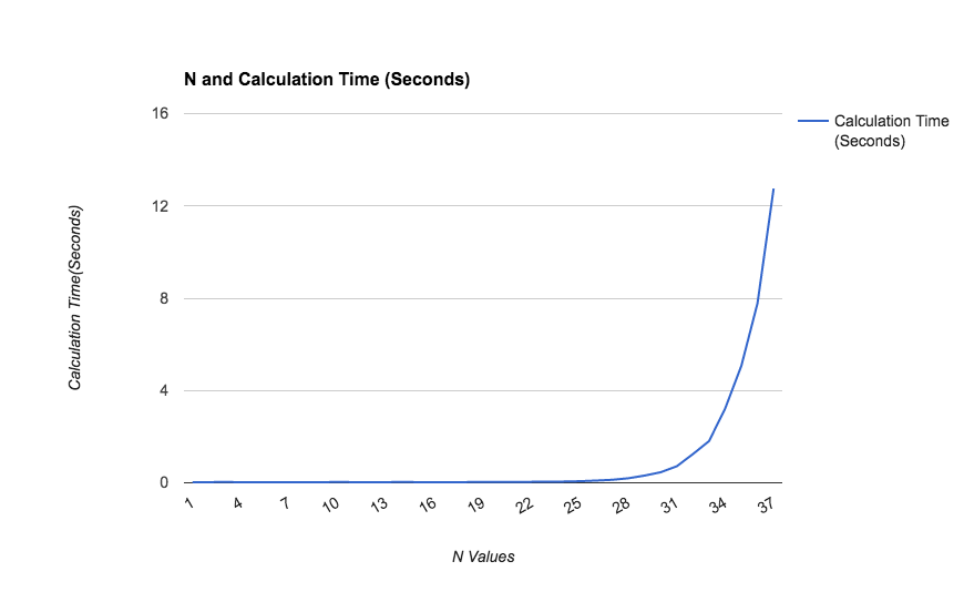
As you can see, the required time to calculate the Nth Fibonacci value increases exponentially as N increases. If we are interested in calculating any large Fibonacci numbers, we’re going to be waiting a very long time, which is impractical.

It’s fairly easy to calculate the first few numbers - but what if we need to calculate the first ten thousand? Certainly a big concern is the size of the numbers themselves, but as we can see, we have an even more immediate problem. Our calculation time seems to be increasing exponentially even with N values as low as 35.

Computer Scientists use several notations (called “Asymptotic Notations”) to describe algorithms, in order to reason about how the computation time can change depending on the input to the algorithm. One such notation - a very popular example - is “Big O”.

There are certainly several factors that can affect the performance of an algorithm, such as the type of hardware being used, the efficiency of the compiler used to compile the source code, etc. However, asymptotic notations like Big O are predicated on the idea that we can ignore some of these messy details in order to describe algorithmic performance at a high level and solve some of the larger problems.

Big O notation intentionally throws away inconsequential constants, providing a cleaner notation. A good example of this is including calculations for things that always take a constant amount of time - in other words, things that are not directly influenced by the input to the algorithm. For instance, if your algorithm always initializes an array of size N before doing any work, that operation does take some time, but the amount of time it might take only increases at a constant rate. Therefore:

O(3n) = O(n)

O(n) sounds good, but is it? What if N is 10 trillion? Don’t fall into the trap of believing that a runtime that was good for one problem is good for another. A big-picture understanding of the problem space is still highly relevant.

It’s not exact, and it’s not meant to be. Big O notation is meant to give us a “big picture” overview of the performance of a certain algorithm.

Note that you might also hear “worst case” vs “best case” within the context of Big O. This refers to the fact that an algorithm can receive a wide variety of input - both very small (which tends to not illuminate performance problems) to very large. In my experience, if this is not explicitly mentioned, the Big O notation refers to “worst case” scenario, such as the largest possible input to an algorithm. This is because “worst case” tends to really show any performance problems in an algorithm.

Big O is a “first line of defense” in our optimization journey. If we’re at the point where we need to worry about making “constant” level improvements (things that shave nanoseconds off a computation) then we’re already beyond Big O notation. Think “Big O helps us solve big problems”.

Big O Analysis

Let’s take a look at some examples and determine our computational complexity in terms of Big O.

If an operation within an algorithm simply does not change it’s behavior based on input, we can notate that easily as well. For instance, many functions return a value. This is a one-time operation, since it serves as an exit point for a function. This means that the value of our input N does not have an impact on how many time this runs. We can say that a “return” statement runs at :

O(1)

A dead giveaway for a basic performance issue is when you see nested code that is dependent on input. For instance, take the following Python example that calculates the maximum difference between two splits of an input list.

def maxdiff(N):
    """Calculates max difference between two splits of an input list (N)
    """

    biggest_diff = 0
    k = 1

    # This loop runs at O(input_list) because in the worst-case scenario,
    # it must iterate over the length of the entire list
    while k < len(input_list):

        # Python's "max" function also iterates over
        # the input list; it runs at O(input_list)
        # in this case
        left_max = max(input_list[:k])
        right_max = max(input_list[k:])

        this_diff = abs(left_max - right_max)

        if this_diff > biggest_diff:
            biggest_diff = this_diff

        k += 1

    return biggest_diff

As noted by comments in the code above, the outer loop runs over the length of the input list “input_list”. This means, the outer loop runs in O(N) time, where N is the “input_list” parameter.

In addition, within this loop, the built-in Python function max() is called twice, once on each part of the list that’s been split up. This ends up roughly running in O(N) time as well. Since this is nested within the loop that’s already running at O(N) time, we say that the maxdiff function runs at O(n^2) time, which is not great. This means that the time it takes to calculate the result will grow exponentially as the length of the input list increases. Eventually, for longer and longer inputs, this time will become infeasible.

We can now turn our attention back to the fibonacci example from earlier in this post, which is clearly a very poorly optimized algorithm. We can be fairly confident that recursively calling a function to calculate each number in the sequence can get way out of control, fast. But how fast?

If you try to visualize recursion, most often what you come up with is some kind of tree structure. A canonical “interview question” example of recursion is to write a program that recursively looks through a tree to do some work.

What we’re doing here is not far off. Every time we run the “get_fib_at_n” function, it kicks off two more instances of itself. It does this until n == 1, in which case the recursion stops, and each instance returns its calculated value.

This means that if we were to visualize this process in a tree, each node, or decision point, where n is not yet 1, has two nodes branching off of it. Also, the leaf nodes at the bottom, always equal 1, since that’s the “exit condition” from this recursive process.

          n       
       /     \
      n-1     n-2     -------- maximum 2^1 additions
     /  \     /   \
   n-2  n-3  n-3 n-4  -------- maximum 2^2 additions
  /   \           
 n-3 n-4              -------- maximum 2^3 additions           

Credit StackOverflow(http://stackoverflow.com/questions/7547133/why-is-the-complexity-of-computing-the-fibonacci-series-2n-and-not-n2)

Our constant “2” is there to illustrate the fact that we are performing two operations in order to get the sum - but the number of times that operation is performed grows exponentially based on N. As you can see from the tree, even by looking at the first 3 layers, the complexity grows at a rate of 2^(n-1). In Big O notation, the exponent can be simplified, and we say this algorithm runs at:

O=2^n

This runtime is atrocious - and it means we can’t practically use this algorithm as implemented.

Fibonacci Algorithm - Optimized

There are many ways to fix problems like this, which depend greatly on the problem being solved. For our Fibonacci example, we can simply store the calculated numbers in a Python list, and within our loop, simply refer two the last two items in the list.

def main():

    fibSequence = []

    try:

        # "n" is the position within the fibonacci
        # sequence that we wish to retrieve
        N = int(sys.argv[1])

    except IndexError:
        print("Please provide N")
        sys.exit(1)
    except ValueError:
        print("Please provide an integer for N")
        sys.exit(1)

    for i in range(N):
        if i <= 1:
            this_number = 1
        else:
            this_number = fibSequence[-1] + fibSequence[-2]

        # This is an example of memoization - storing the result of
        # a calculation so that in the future, the calculation doesn't
        # need to be repeated
        fibSequence.append(this_number)

    print(fibSequence[-1])

if __name__ == "__main__":
    main()

Python performs such list lookups in constant time, which means that this algorithm runs in O(N), due to the loop. This is a much more feasible runtime.

We solved this particular problem using a technique called “memoization”. This is a common technique to consider when optimizing algorithms. In short, with memoization we store calculated values and refer to them later, instead of recalculating them repeatedly and unnecessarily.

If you’re recalculating the same value, or if parts of your logic is directly influenced by the size of N, it’s worth re-evaluating your algorithm to see if memoization can help keep things efficient.

Striking a Balance

You might also hear about two types of complexity that’s described by Big O. Time complexity is one that we’ve already discussed in detail. Our first Fibonacci algorithm ran in O(2^n) time, for instance.

However, Big-O can also be used to describe storage complexity. If your program doesn’t clean up memory resources, or isn’t careful about what it stores, the same problems can be realized from a storage capacity perspective (both with repect to capacity as well as speed of access).

We created that first Fibonacci example because we feared that storing these values might present a storage problem - but this fear was not driven by data. It turns out that it’s far less costly to store the fibonnaci values than to recursively calculate them on the fly.

To be fair, eventually we would run out of space, so if you wanted to take this example even further, you don’t have to store all of the Fibonacci values in memory - you really only need a pair of values, in order to calculate the 3rd. Once the 3rd has been reached, you can discard the 1st value, and you have two new values.

Algorithm design is all about being aware of the tradeoffs you’re making, and striking the right balance. Be aware of this for both computational complexity as well as storage complexity.

Algorithmic Approaches

There are a number of approaches that you can take when trying to solve a problem with an algorithm. I won’t explore all of them, but will enumerate a few here.

Once popular choice is “divide and conquer”, which divides a problem into a subset of smaller problems that are easier to deal with. This approach often results in some kind of recursive solution, since you likely want to perform the same logic on the sub-problem, as you did on the larger problem.

A good example of this is the “merge sort”. This is a sorting technique which cuts the input set in half, and then merges the two halves together in the right order. Despite the fact that this solution usually leverages recursion, each level reduces the input by cutting it in half. As a result, a merge sort generally runs in O(n log n) time, which is a lot better than O(2^n)

There are many other approaches, each of which is not necessarily “better” than the others - but rather are more suitable for a certain type of problem. It’s important to be aware of all of these, and consider them when looking at designing your own algorithm.

Testing Techniques

When writing an algorithm, you should definitely test it. Take a sort of “hacker” approach to the problem - really put your algorithm to the test, and try to see where it breaks.

I tend to write some function that randomly generates values of a size that I determine using arguments. For instance, you may have an idea of a reasonable input that your algorithm may be subjected to. I wrote a “gen_testdata” function that takes such parameters, and generates a random list of integers that I can then run an algorithm on - perhaps a sorting algorithm:

import random


def gen_testdata(lower, upper, upper_len, lower_len=0):
    """Produces a randomized list of integers

    This is useful for testing algorithms - feed it some of this data
    and watch it melt
    """

    list_len = random.randint(lower_len, upper_len)

    ret_list = []

    for i in range(list_len):
        ret_list.append(random.randint(lower, upper))

    return ret_list



def main():

    # We can feed in the boundaries for our test data as parameters
    # to the function that generates test data, so we know
    # within what limits our algorithm performs
    sample_data = gen_testdata(-39487, 45984, 10000)

    start = datetime.now()
    thissolution = awesome_algorithm(sample_data)
    done = datetime.now()
    print "Solution is: " + str(thissolution)
    elapsed = done - start
    print "Computation time: %s seconds" % (
        elapsed.total_seconds()
    )

if __name__ == "__main__":
    main()

You’ll also notice that I am taking a timestamp immediately before and after I run the “awesome_algorithm” function, so I know how long it took to run.

In addition, if you’re concerned about memory footprint, the third-party Python package “memory_profiler” is quite popular. The usage is quite easy - once we import the package, we can add a simple decorator to the top of our algorithm:

from memory_profiler import profile

@profile
def awesome_algorithm():
    ...

When we run this code, we get a nice report printed to the shell:

~$ python test_profile.py
Filename: test_profile.py

Line #    Mem usage    Increment   Line Contents
================================================
    66      8.9 MiB      0.0 MiB   @profile
    67                             def awesome_algorithm():
    68      8.9 MiB      0.0 MiB       test_list = []
    69
    70      8.9 MiB      0.0 MiB       for i in range(100):
    71      8.9 MiB      0.0 MiB           test_list.append(i * 2)
    72
    73      8.9 MiB      0.0 MiB       return test_list

Once you have a handle on how exactly you want to test your particular algorithm, it’s super common to run those tests within some kind of unit test, which can be run automatically by your Continuous Integration service (which you’re totally using, right?). This way you know that your algorithm is holding up to your tests when you change it.

Conclusion

Here are some great resources that you should definitely check out to take your understanding of algorithms further:

• Algorithmic Toolbox on Coursera - I took this, and it is a great introduction to algorithms.
• Big O Cheat Sheet - amazing collection of algorithms and their runtimes for quick reference
• Algorithm Visualizer - There is also a hosted version of this, but it’s not always online. Hopefully it is for you. VERY handy and FUN tool!

There are many more details involved with the study of algorithms, including additional asymptotic notations in addition to “Big O”, but this is a good starting point.

You may be asking yourself - why does any of this matter? You may not be interested in software development, or perhaps you’re just getting started, and with today’s open source ecosystem, it’s likely that these kind of low-level concepts are already implemented in some kind of library that you can simply re-use, right?

The study of algorithms is still useful. It matters becuase it’s helpful to be thinking about things in terms of algorithms and ensuring that you are making the right tradeoffs. Sometimes, optimizing a piece of code is worth it - sometimes it is not. Educating yourself on the tradeoffs (and communicating them well in documentation) is a worthwhile exercise.

Even if you’re not a software developer - algorithms are all around you. They are at the core of every piece of technology you interact with daily.