Classifying MNIST Handwritten Digits With a Fully Connected Neural Network
December 28, 2025 in Machine Learning18 minutes
I’d like to continue on my deep learning journey. In my first blog on this topic I built a basic neural network “from scratch”. This was done intentionally to learn how things work at a low-level, even though it was impractical for any “serious” usage.
So I’d like to level things up a bit in a few ways. One, I’d like to learn more off-the-shelf tooling that is already widely used, such as PyTorch (eventually I aim to get to others). Now that I understand at least the basics of what these tools are actually doing under the hood, they’ll be less like magic and more like a force multiplier. Two, I want to learn something a bit more practical - image classification is a common early problem to solve, and the hand-written digits in the MNIST dataset is a classic example.
Conventionally this is solved best with convolutions, or Convolutional Neural Networks (CNNs). While I aim to get there soon, I’m going to first make an intermediate step by attempting to do this using a fully-connected topology. This will help me keep the new concepts to a minimum while I also learn the new (to me) tooling. I’m also curious to quantify just how different the fully-connected vs CNN approaches differ in terms of accuracy and other qualities (I’ve heard that convolutions, due to their spatial awareness, are just “better” at this. This makes logical sense but I want to experience it firsthand).
I broke this down into a few discrete steps / functions which will be explained in the sections below.
For brevity, I will not be including explicit code snippets for everything in this blog post, particularly those around visualizations for the data and the training process. Code snippets around more important concepts will still be focused on very relevant portions of code, rather than being contextually complete.
That said, all code used here will be contained within the notebook which can be found at the end of the blog post. So if at any point you’re wondering about how the examples provided actually work together, check that out at the end.
The MNIST Dataset
We’ll be working with the MNIST handwritten digits dataset. This is available via the torchvision package. We’ll be working with the data in batches, so we’ll want to construct a function which returns the data in the form of a loader, which is basically an iterator which gives us the data in the batch size we specify.
We’ll need to return two loaders - one for the training data (which we’ll obviously use to train our network) and the “test data” which will only be used for forward passes after training to determine how well our model is doing at predicting what digit is in a given image.
As part of this loading process we’ll also need to apply a few transformations from the torchvision package to get the datasets ready for our network. The first and arguably most important of these is to convert the dataset from their native format (PIL images) to PyTorch tensors. Fortunately there’s a simple one we can simply use called ToTensor() which does this for us. It also adjusts the value range from this native format (0 to 255) to 0-1, which will be helpful to align with the activation we’ll use - most of these center around this range.
Skipping ahead a little bit, and with a bit of matplotlib magic, we can visualize the data within a given batch from the training dataloader:
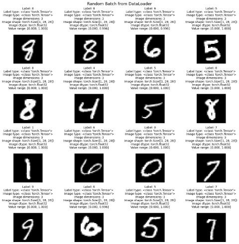
From this, we learn that the images are 28x28 pixels. However, as you can see they’re reported as [1, 28, 28] by pytorch, the first value of which represents the channel (in this case a black-and-white image, so it’s a single channel. An RGB image would have 3 here). We can also see that the range is that which resulted from our ToTensor() transformation - 0 to 1.
Another useful transformation to consider is Normalize. In deep learning the process of normalization involves centering and scaling the data to make the gradient descent more predictable and efficient.
The MNIST handwritten dataset is already pretty well-behaved and only considers a single feature (the 0-1 per-pixel greyscale value), so the value of normalizing here isn’t nearly as significant as it would be for other more complex problems.
However, there’s no harm in doing it in this case, and is a good concept to be familiar with for more complex problems that involve tracking multiple features with wildly different scales.
To do this, we can pop in the well-known mean and standard deviation values for the MNIST dataset:
The resulting tensors will instead be centered with a mean of approximately 0, and a standard deviation of approximately 1.
A more complete example of these transformations as they’re applied to the dataloaders is shown below:
 1import torch
 2import matplotlib.pyplot as plt
 3import torchvision
 4import torchvision.transforms as transforms
 5
 6def load_data(batch_size, normalize=True, shuffle=True):
 7
 8    # Transformations to apply to both datasets.
 9    transform=transforms.Compose([
10        # Converts a PIL Image or numpy.ndarray (H x W x C) in
11        # the range [0, 255] to a torch.FloatTensor of shape
12        # (C x H x W) in the range [0.0, 1.0]
13        transforms.ToTensor(),
14        # This standardizes each tensor with a given mean and
15        # standard deviation. (the values provided here are
16        # the mean and std deviation for the MNIST dataset)
17        transforms.Normalize((0.1307,), (0.3081,))
18    ])
19
20    # Load the datasets
21    train_dataset = torchvision.datasets.MNIST(
22        root='./tmp',
23        train=True,
24        download=True,
25        transform=transform
26    )
27    test_dataset = torchvision.datasets.MNIST(
28        root='./tmp',
29        train=False,
30        download=True,
31        transform=transform
32    )
33
34    # Create DataLoaders for batching and shuffling
35    train_loader = torch.utils.data.DataLoader(
36        train_dataset,
37        batch_size=batch_size,
38        shuffle=shuffle
39    )
40    test_loader = torch.utils.data.DataLoader(
41        test_dataset,
42        batch_size=batch_size,
43        shuffle=False
44    )
45    return train_loader, test_loader
We now have our dataloaders and can move on to designing our network.
Network Design
There are a number of design considerations to ponder before we throw a network together. The first is about the general topology. We know we need an input layer composed of 784 neurons (one per pixel in a flattened 28x28 image), and it’s reasonable to assume we’ll need 10 neurons in our output layer (so we can have our network provide % confidence for each possible value of 0 - 9) but what does the rest of the network look like? How many hidden layers, and how many neurons per layer?
To me, perhaps because I’m still new, these questions have not had a deterministic answer. Most of what I’ve seen indicates that starting with something “reasonable” and iterating from there is as good as anything else. So I’ll be starting with two hidden layers - each of which has 512 - and go from there.
Why 2x512? both seemed like reasonable “even” numbers, close-ish to the size of our input layer. My plan is to build the actual implementation of this network to easily parameterize this topology so I can tweak them along with other hyperparameters, and observe the impact on training, and the resulting model’s accuracy.
In a future blog post I intend to more directly answer this question I still have about not really having any “design instincts” in this phase of things that can be applied to different kinds of problems. It would seem to me that I should have some first principles to rely on here rather than “that number sounds good”, but I haven’t discovered them yet.
The other important consideration is the activation function to use. While my prior post used sigmoid, I’ve since learned that “recified linear unit” or “ReLU” is far more widely used today. One reason for this is that it’s remarkably simple. It simply outputs the input as-is if it is positive, otherwise it outputs 0.
$$ f(x)=\max(0,x) $$This works well for 0-centered datasets (which we’ve done during normalization) because by definition half our neurons will be activated - a great place to be when starting the training loop. While not totally impervious to all problems, it also doesn’t have the same kind of “vanishing gradient” problem that others like sigmoid can have.
 1from torch import nn
 2
 3class Network(nn.Module):
 4    def __init__(self, layer_sizes):
 5        super().__init__()
 6
 7        # We're using a fully connected network here, which will use
 8        # https://docs.pytorch.org/docs/stable/generated/torch.nn.Linear.html
 9        # This requires a 1D vector, so we need to convert our
10        # 28x28 grid to a 1D vector of 784 values.
11        self.flatten = nn.Flatten()
12
13        # Input size is fixed for MNIST (28x28)
14        input_size = 28 * 28
15        # Output size is also fixed (numbers 0-9)
16        output_size = 10
17
18        # Combine input size, hidden layers, and output size into one list
19        sizes = [input_size] + layer_sizes + [output_size]
20
21        # Construct hidden layers
22        layers = []
23        for i in range(len(sizes) - 2):  # all except the last layer
24            layers.append(nn.Linear(sizes[i], sizes[i + 1]))
25            layers.append(nn.ReLU())
26
27        # Add the final output layer (no activation)
28        layers.append(nn.Linear(sizes[-2], sizes[-1]))
29
30        # Wrap in a Sequential block and store for the forward pass to use.
31        self.linear_relu_stack = nn.Sequential(*layers)
32
33    def forward(self, x):
34        x = self.flatten(x)
35        logits = self.linear_relu_stack(x)
36        return logits
Some points about the above:
- As mentioned in a comment, the
Linearlayer requires a 1D vector so we need to flatten our 2D grid. An alternative could be to flatten our dataset before passing it into the network, but since this is all very small, it’s fine to do it here (especially due to the convenience of the provided method). A solution aimed at solving a more complex problem with more data may elect to do more work during the data loading phase, putting less work on the network itself. - I like this pattern from the docs and used it when defining
linear_relu_stack. Doing it this way then simply allows me to call this during theforward()method, rather than redefine it in that method each time. You’ll also notice it’s dynamically generated based on thesizesparameter. As I mentioned earlier, I want to be able to parameterize the network topology so that I can easily run the training loop with different topologies and compare the results. - Choosing initial weight/bias values was a big deal in my previous post. PyTorch does this for us for our
Linearlayers using the approach described in Kaiming et al. This is an initialization method well-suited for our ReLU activation - whereas my previous post which used sigmoid benefitted from Xavier/Glorot initialization
Printing this network after initializing it with sizes of [512, 512] (2 layers, 512 neurons each) yields a quick summary that makes it easier to reason about through the dynamic build logic I added:
Sequential(
  (0): Linear(in_features=784, out_features=512, bias=True)
  (1): ReLU()
  (2): Linear(in_features=512, out_features=512, bias=True)
  (3): ReLU()
  (4): Linear(in_features=512, out_features=10, bias=True)
)
In summary, this creates a network where each of our hidden layers gets a ReLU activation (important for non-linearity) but no matter what the last item in the stack is our Linear output layer. We’ll see why this was important in the next section.
Classification Loss
Next we need to understand how to calculate loss for this network during the training phase. As a reminder from last time, this is a mathematical way to quantify how “wrong” our model’s prediction is. This is important because this loss is used to calculate gradients - a crucial step for training our model to be more accurate.
In pytorch, the term “criterion” is often used interchangeably with “loss function” or “loss module”
CrossEntropyLoss is an established go to for multi-class classification problems like this one (10 classes from 0-9). I plan to get into the math in a later blog post, but one important thing to note is that this loss function uses softmax to convert raw “logits” to a probability distribution.
While hidden layers generally need to pass this value into an activation function to ensure non-linearity, the output layer needs to instead leave these values to remain as-is so that CrossEntropyLoss can do its thing. It is for this reason that we ensured that the last entry in our Sequential stack in the network definition was Linear, instead of ReLU or something else. This ensures that the simple weighted sums from the output layer are made available to our loss function.
Training Loop
It’s now time to construct our training loop. This will be responsible for iterating over all of the batches in the dataset based on a provided batch size.
The load_data function we defined at the beginning included a batch_size parameter. We’ll be using that now as part of an approach known as “mini-batch gradient descent” which computes an average gradient across all samples in a given batch, rather than computing a gradient per-sample. This batch size is configurable, and will be one of the hyperparameters I’ll tweak in the evaluation section.
The “optimizer” is what we’ll use to perform the mini-batch gradient descent. PyTorch comes with a few, but SGD is the one we want in this case. It’s simple, and does much the same thing as I did by hand in my first post.
SGD stands for “stochastic gradient descent” and this naming caused a little bit of confusion for me. There’s nothing inherently stochastic about this optimizer from what I can tell - it’s assuming this has already been done for the batch that’s passed to it - which is true in this case.
The loader we already defined is responsible for randomly selecting samples from the training data based on our batch size. SGD will calculate an average gradient for this batch.
With these selections made, we can now define the loop. This loop will iterate over the dataloader, and on each iteration will process a batch of the size we select when we invoke this function. Within each iteration, a series of ordered steps take place:
- Perform a forward pass on each batch - getting back a tensor containing predictions for each image
- Calculate the average loss for the entire batch
- Calculate the gradient based on this loss and backpropagate into the model
More details about each step and the implementation specifics are below:
 1def train_loop(dataloader, model, learning_rate, batch_size=64):
 2
 3    # Defaults to reduction='mean' which means it will provide an average
 4    # loss for the entire batch
 5    loss_fn = nn.CrossEntropyLoss()
 6
 7    # model.parameters() gives the optimizer a generator containing references
 8    # to the tensors of the model containing the weights and biases.
 9    optimizer = torch.optim.SGD(model.parameters(), lr=learning_rate)
10
11    # So we can show % progress as we iterate over the dataset
12    total_size = len(dataloader.dataset)
13
14    # Set the model to training mode - important for batch normalization and
15    # dropout layers. Unnecessary in this particular situation but added
16    # for best practices
17    model.train()
18    for batch_idx, (images, labels) in enumerate(dataloader):
19        # Forward pass - the model (and loss_fn) both receive the entire batch at once
20        pred = model(images)
21        loss = loss_fn(pred, labels)
22
23        # PyTorch by default accumulates gradients on each tensor.
24        # We don't want/need that for this, so we make sure we zero out
25        # the gradients before calling `loss.backward()`
26        #
27        # https://docs.pytorch.org/tutorials/recipes/recipes/zeroing_out_gradients.html
28        optimizer.zero_grad()
29
30        # This calculates the gradient for each weight tensor and stores the result on
31        # its `.grad` attribute
32        #
33        # https://docs.pytorch.org/docs/stable/generated/torch.Tensor.backward.html#torch.Tensor.backward
34        loss.backward()
35
36        # This actually applies the gradient calculated above by `loss.backward()`
37        #
38        # https://docs.pytorch.org/docs/stable/generated/torch.optim.SGD.html#torch.optim.SGD.step
39        optimizer.step()
40
41        # Print progress/loss every 100 batches
42        if batch_idx % 100 == 0:
43            loss, current = loss.item(), batch_idx * batch_size + len(images)
44            print(f"loss: {loss:>7f}  [{current:>5d}/{total_size:>5d}]")
Eval and Epoch Loops
Next, we need a greater epoch loop from which the training loop is called. If the training loop iterates over all mini-batches in a dataset, we need a greater loop from which the training loop can be called, so we can repeat the entire training loop as many times as is necessary to get a well-trained model.
Before we can do this, we need to define one more loop - the “eval loop”. This will iterate over batches in the test dataset and evaluate the model’s prediction accuracy in a purely “evaluation” (i.e. “non-training”) mode. We’ll use this to judge the real accuracy of our model after each epoch.
 1def eval_loop(dataloader, model):
 2
 3    loss_fn = nn.CrossEntropyLoss()
 4
 5    # Set the model to evaluation mode - important for batch normalization
 6    # and dropout layers. Not totally required in this situation but added for best
 7    # practices
 8    model.eval()
 9    total_size = len(dataloader.dataset)
10    num_batches = len(dataloader)
11
12    # We will be returning the average loss and accuracy for
13    # the predictions in this loop - start the counters at 0
14    test_loss, correct = 0, 0
15
16    # Evaluating the model with torch.no_grad() ensures that no gradients are
17    # computed during test mode. Also serves to reduce unnecessary gradient
18    # computations and memory usage for tensors with requires_grad=True
19    with torch.no_grad():
20        for images, labels in dataloader:
21            pred = model(images)
22            test_loss += loss_fn(pred, labels).item()
23            correct += (pred.argmax(1) == labels).type(torch.float).sum().item()
24
25    # convert to averages and return
26    test_loss /= num_batches
27    correct /= total_size
28    return (test_loss, correct)
This function returns the average loss and accuracy.
This loop is fairly simple, and it’s where we start to tie together what we’ve already built so far. After calling load_data to get our train and test loaders, we’ll iterate for num_epochs, and run through the training loop on each invocation.
After the training loop, we’ll also run the eval loop - once for the training dataset, and another for the test dataset. This is an important step to help detect if overfitting is taking place.
 1def epoch_loop(layer_sizes, num_epochs, learning_rate, batch_size):
 2
 3    print(f"Starting new epoch loop with layer_sizes: {layer_sizes}, " +
 4          f"num_epochs: {num_epochs}, learning_rate: {learning_rate}, batch_size: {batch_size}")
 5
 6    model = Network(layer_sizes)
 7    train_loader, test_loader = load_data(batch_size)
 8
 9    for epoch in range(num_epochs):
10        print(f"Epoch {epoch+1}\n-------------------------------")
11
12        train_loop(train_loader, model, learning_rate)
13
14        # To help detect overfitting, we want to run the same eval loop which is used for the test
15        # dataset against the training dataset as well, but only after the training loop has completed.
16        #
17        # This ensures we're comparing the two equally, and helps us detect overfitting.
18        train_loss, train_acc = eval_loop(train_loader, model)
19        test_loss, test_acc = eval_loop(test_loader, model)
20
21        print(f"\nTrain - Accuracy: {(100*train_acc):>0.1f}%, Avg loss: {train_loss:>8f}")
22        print(f"Test - Accuracy: {(100*test_acc):>0.1f}%, Avg loss: {test_loss:>8f} \n")
Iteration and Insights
Now that we have our epoch loop, it’s time to actually call it - and determine which hyperparameters have the most positive impact on our model’s performance. We’ll experiment with different architectures (depth/width), different learning rates, different batch sizes, etc.
To help facilitate this process, I’ve defined a few extra functions for visualizing this process for each invocation. One will plot training and eval accuracy plus loss over time (epochs). This will be crucial for understanding when the model’s training is plateauing, and/or if overfitting is taking place.
First Attempts
As mentioned previously, we’ll start with two hidden layers of 512 neurons each. We’ll run for 20 epochs, with a batch size of 64, and a learning rate of 0.001. All of these are parameters to epoch_loop so we can do all this by simply invoking:
1epoch_loop(layer_sizes = [512, 512], num_epochs=20, learning_rate=1e-3, batch_size=64)This design appears to get test accuracy up to only about 89.4%. The full performance graph can be seen below:
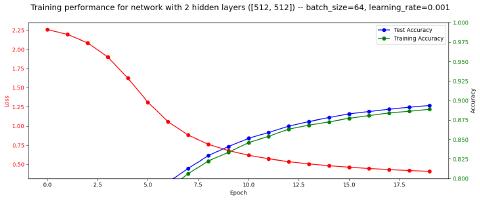
The graph has a y-axis minimum of 0.8 to ensure we can see more clearly where the accuracy ends up at the end of the epoch loop
A few thoughts:
- Even though 20 epochs is fairly generous, and plateauing is starting to take place, it’s clear that more epochs could result in a higher accuracy (or other changes could be made to increase accuracy more quickly).
- No overfitting appears to be taking place - training accuracy consistently lags behind test accuracy by about 0.4% - I am hypothesizing that this has to do with the training set being much larger, with more difficult edge cases. So this feels to me the right direction - the model is generalizing as desired.
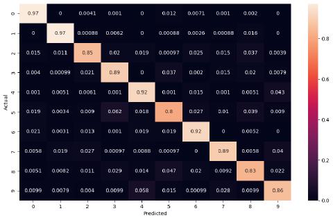
The “confusion matrix” for this first attempt is quite interesting - with digits like 0 and 1 showing 97% prediction accuracy, and others like 5 showing low 80%.
Continuing to Tweak
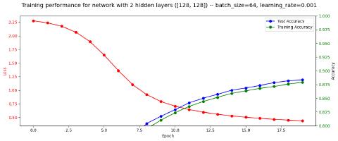
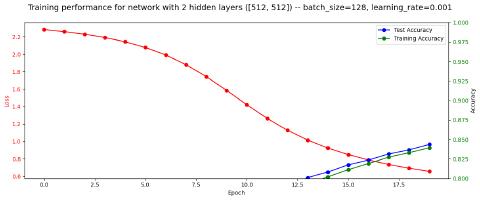
In subsequent attempts I tweaked various hyperparameters and other settings and saw some slight differences in performance:
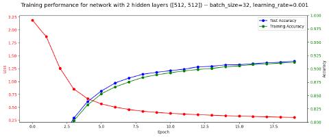
However, the largest improvements came from increasing the learning rate and reducing the batch size:
Final Results
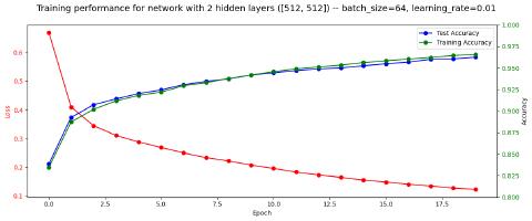
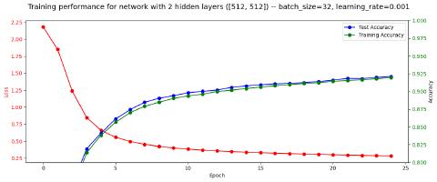
For my best attempt, I combined the two most significant improvements by picking a middle-ground learning rate, and using the batch size of 32:
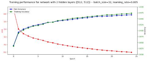
Observations:
- Definitely the best accuracy so far, and surprisingly high. I wasn’t expecting the fully connected approach to get as high as ~98%
- My initial understanding of overfitting had me worried about the “crossover” at about epoch 7. However I believe this is all normal, as both training and testing accuracy steadily increased up through the final epoch.
Conclusion
I found this exercise to be useful for refreshing the knowledge I already had from my first “from scratch” post, familiarizing myself with pytorch, and pushing me into learning new things as I scale things up like mini-batch gradient descent and cross-entropy loss.
From my initial reseach on this common “hello world” problem for image classification, I got the impression I wouldn’t be able to get anywhere near the accuracy I did with the fully-connected approach. Since I was able to get up to ~97%, I’m wondering if convolutions can push to really high accuracy, perhaps even 99.9% or even higher. I am looking forward to exploring this in a follow-up post.
All of the code used for this analysis can be found below.
View this marimo
notebook below (best on desktop), or in a separate tab.
Note: Due to environment limitations, this notebook is read-only and not interactive. You must download and run locally.
